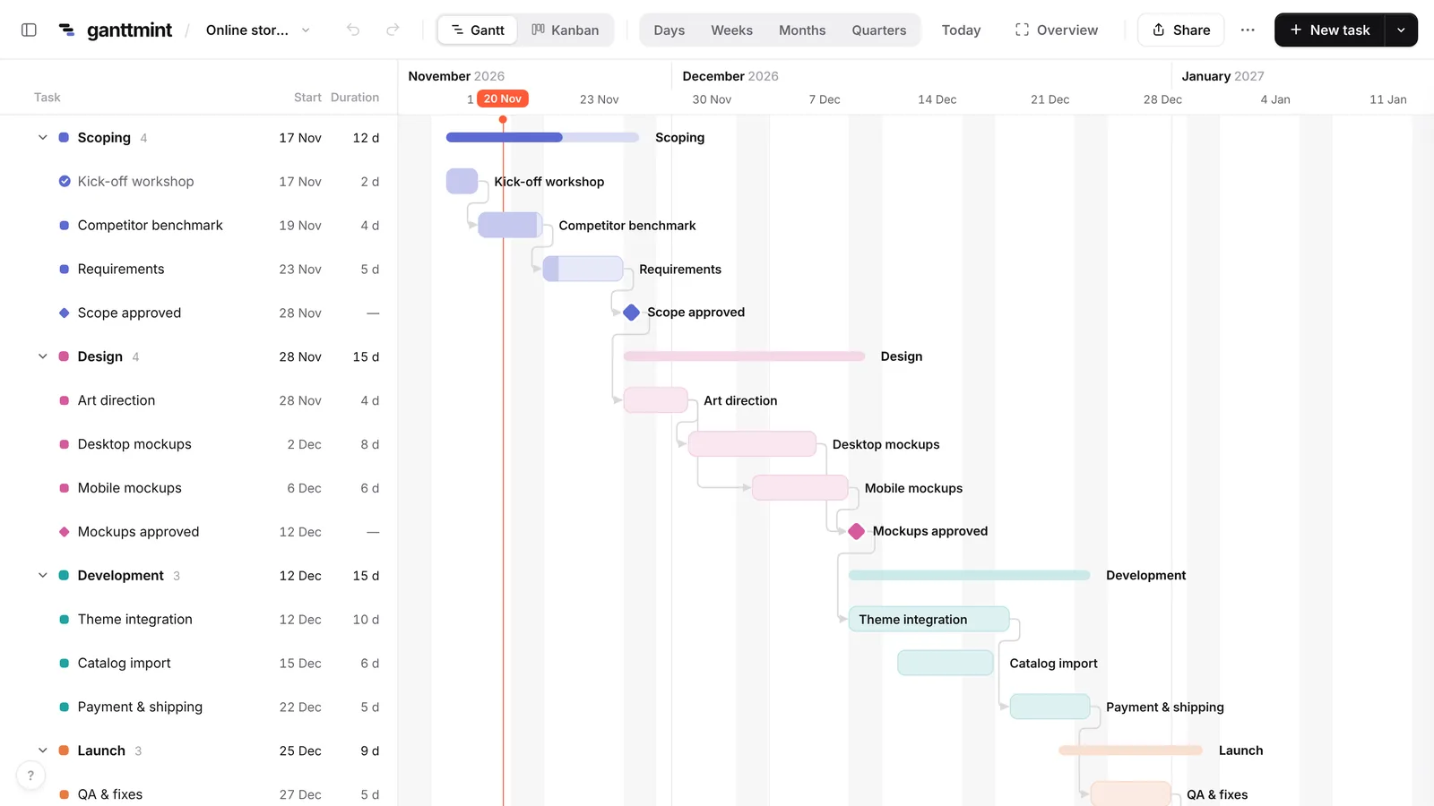
Excel doesn’t have a Gantt chart type. You can still build one in about fifteen minutes, and this guide shows the two methods that work: a stacked bar chart (the classic) and conditional formatting (easier to keep up to date). At the end you’ll find a free Excel Gantt chart template, and a faster way to do the same thing online.
What you need before you start
A Gantt chart is just a list of tasks drawn on a timeline. For each task you need three things:
- a task name,
- a start date,
- a duration in days (or an end date, and Excel calculates the duration).
Put them in a table, one task per row, with headers in row 1: Task, Start, End, Duration. In the Duration column, use =C2-B2+1 so it updates when you change a date.
Method 1: a stacked bar chart
This is the method most tutorials show. The trick is to draw two bars per task, an invisible one that ends at the start date and a visible one for the duration.
- Select the Start column (B1 to the last row), then go to Insert → Charts → Bar → Stacked Bar.
- Add the durations: right-click the chart, choose Select Data, click Add, name the series
Durationand select the Duration cells as values. - Show task names on the axis: still in Select Data, edit the horizontal (category) axis labels and select the Task column.
- Hide the first series: click the blue bars (the start dates), open Format Data Series and set Fill to No fill. Only the duration bars remain.
- Put the first task at the top: right-click the vertical axis, Format Axis, and tick Categories in reverse order.
- Remove the empty space at the left: Excel starts the date axis in 1900. Select your first start date, change its format to Number to see its serial number (something like
46346), then put that number in Format Axis → Bounds → Minimum for the horizontal axis. Switch the cell back to a date afterwards. - Make it readable: set Gap Width to about 40 % so the bars get thicker, and delete the legend.
You now have a Gantt chart. It works, but it has real limits: there are no dependencies between tasks, milestones need workarounds, and every time a task slips you have to shift the dates that follow by hand.
Method 2: conditional formatting (easier to maintain)
Instead of a chart, you colour cells in a grid of dates. It’s more robust because the chart is just your table.
- Keep your table in columns A to D.
- In row 1, starting from column F, write the dates of your project: put the first date in F1, then
=F1+1in G1 and drag it to the right for as many days as you need. - Select the grid area (F2 to the last column and row), then go to Home → Conditional Formatting → New Rule → Use a formula.
- Enter
=AND(F$1>=$B2,F$1<=$C2)and pick a fill colour.
Each task now lights up across the days it covers. Change a date in column B or C and the bar moves on its own. To show weeks instead of days, use =F1+7 in step 2 and adapt the rule to =AND(F$1+6>=$B2,F$1<=$C2).
Download a ready-made Excel Gantt chart template
If you’d rather skip the setup, our free Gantt chart templates come as Excel files. The timeline is built with formulas: change a start date or a duration and the bars move by themselves. There are templates for a project plan, a product launch, a website project and event planning.
Where Excel falls short
Excel is great for a one-off plan you print once. It gets painful when the project is alive:
- Dependencies: if the design is late, Excel doesn’t push development back. You do it, row by row.
- Zooming out: going from days to months means rebuilding the grid or the axis.
- Sharing: you end up emailing
plan_v7_final_FINAL.xlsx, and nobody knows which version is current. - Kanban: the people doing the work often prefer a board of cards. In Excel that’s a second file to keep in sync.
The faster way: make your Gantt chart online
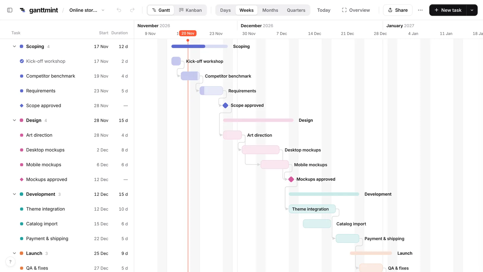
Ganttmint is a free online Gantt chart maker. There’s no account to create and nothing to install: open it, type your tasks, and drag the bars.
- Linked tasks: drag a bar and the tasks that depend on it follow.
- Zoom out in one click: days, weeks, months or quarters, so you keep the big picture.
- Kanban view: the same tasks as cards, sorted by status, always in sync with the Gantt.
- Excel in and out: import your existing spreadsheet, and export to Excel, PNG or PDF whenever you need.
- Share a link: send a read-only link instead of an attachment. It updates as you work.
Already have your plan in Excel? Open the app, choose Import, and select your .xlsx or .csv file. Ganttmint recognises the Task, Start, End and Duration columns automatically.
Not tied to Excel? See how to make a Gantt chart with any tool, or how to make a timeline in Excel.
Quick answers
Does Excel have a Gantt chart template? Microsoft offers a few in File → New, but they are built on the same stacked bar trick, with the same limits. Our templates use formulas so the timeline updates itself.
How do I add a milestone in Excel? The simplest way is a task with a duration of 1 and a different colour. In Ganttmint, press M to add a real milestone.
Can I make a Gantt chart in Google Sheets? Yes, the conditional formatting method works the same way in Google Sheets. You can also learn what a Gantt chart is and how to read one before you start.